YOLO V1 Implementation
YOLOv1 implementation based on the original paper 1
How Yolo works
YOLO is an object detection algorithm and uses features that learned from a CNN network to detect objects. When performing object detection we want to correctly identify in the image the objects in the given image. Most of the classic approaches in the object detection algorithms using the sliding window method where the classifier is run over evenly spaces locations over the entire image. Such types of algorithms are the Deformable Parts Models (DPM), the R-CNN which uses proposal methods to generate the bounding boxes in the given image and then run the classifier on the proposed bounding boxes. This approach, and particularly the DPM method is slow and not optimal for real time uses, and the improved version of R-CNN models is gaining some speed by strategically selecting interesting regions and run through them the classifier.
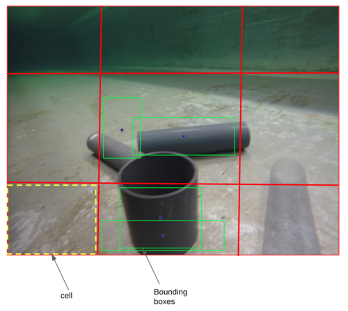
On the other hand YOLO algorithm based on the idea to split the image in a grid, for example for a given image we can split it in a 3 by 3 grid (SxS = 3x3) which gives as 9 cells. As the below image shows, the image consists by a 3 by 3 grid with 9 cells, and each cell has 2 bounding boxes (B) which finally will give the prediction bounding boxes for the object in the image.
Generally, the YOLO algorithm has the following steps:
- Divide the image into cells with an SxS grid
- Each cell predicts B bounding boxes (A cell is responsible for detecting an object if the object's bounding box is within the cell
- Return bounding boxes above a given confidence threshold. The algorithm will show only the bounding box with the highest probability confidence (e.g. 0.90) and will reject all boxes with less values than this threshold.
Note: In practice will like those larger values of $S and B$, such as $S = 19$ and $B = 5$ to identify more objects, and each cell will output a prediction with a corresponding bounding box for a given image.
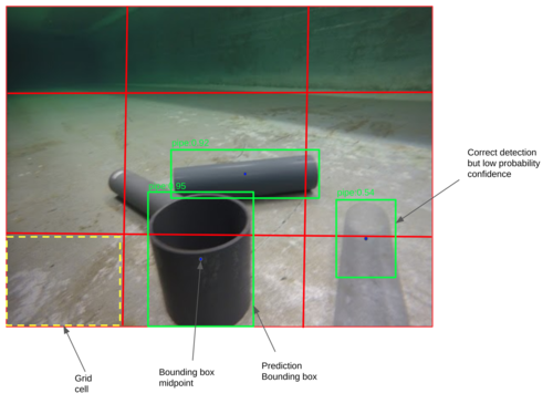
The below image shows the YOLO algorithm's result, which returns the bounding boxes for the detected objects. For the algorithm to perform efficiently needs to be trained sufficiently because with each iteration (epoch), the detection accuracy increases. Also, the bounding boxes can be in more than one cells without any issue, and the detection is performed in the cell where the midpoint of the bounding box belongs.
The YOLO object detection algorithm is faster architecture because uses one Convolutional Neural Network (CNN) to run all components in the given image in contrast with the naive sliding window approach where for each image the algorithm (DPM, R-CNN etc) needs to scan it step by step to find the region of interest, the detected objects. The R-CNN for example needs classify around 2000 regions per image which makes the algorithm very time consuming and it's not ideal for real time applications.
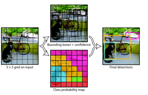
The figure below shows how the YOLO model creates an $S x S$ grid in the input image and then for each grid cell creates multipe bounding boxes as well as class probability map, and at the end gives the final predictions of the objects in the image.
How the bounding boxes are encoded in YOLO?
One of the most important aspects of this algorithm is the it builds and specifies the bounding boxes, and the other is the the Loss function. The algorithm uses five components to predict an output:
- The centre of a bounding box \(bx by\) relative to the bounds of the grid cell
- The width \(b_w\)
- The height \(b_h\). The width and the height of the entire image.
- The class of the object \(c\)
- The prediction confidence \(p_c\) which is the probability of the existence of an object within the bounding box.
Thus, we, optimally, want one bounding box for each object in the given image and we can be sure that only one object will be predicted for each object by taking the midpoint of the cell that is responsible for outputting that object.
So, each bounding box for each cell will have \(x1, y1, x2, y2\) coordinates where in the YOLO algorithm will be \(x, y, w, h\)
\(x\) and \(y\) will be the coordinates for object midpoint in cell -> these actually will be between \(0 - 1\)
\(w\) and \(h\) will be the width and the height of that object relative to the cell -> \(w\) can be greater than 1, if the object is wider than the cell, and \(h\) can also be greater than 1, if the object is taller than the cell
The labels will look like the following:
$$label_{cell} = [c_1, c_2, ..., c_5, p_c, x, y, w,h]$$
where:
- \(c_1\) to \(c_5\) will be the dataset classes
- \(p_c\) probability that there is an object (1 or 0)
- \(x, y, w,h\) are the coordinates of the bounding boxes
Predictions will look very similar, but will output two bounding boxes (will specialise to output different bounding boxes (wide vs tall).
$$pred_{cell} = [c_1, c_2, ..., c_5, p_{c_1}, x_1, y_1, w_1, h_1, p_{c_2}, x_2, y_2, w_2, h_2]$$
Note: A cell can only detect one object, this is also one of the YOLO limitations (we can have finer grid to achieve multiple detection as mentioned above.
This is for every cell and the target shape for one image will be \(S, S, 10\) where:
- \(S * S\) is the grid size
- \(5\) is for the class predictions, \(1\) is for the probability score, and \(4\) is for the bounding boxes
The predictions shape will be \(S, S, 15\) where there is and additional probability score and four extra bounding box predictions.
The model architecture
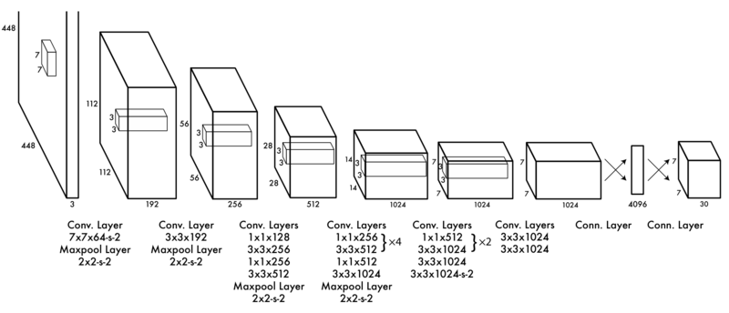
The original YOLO model consists of 24 convolutional layers followed by 2 fully connected layers.
The model accepts 448x448 images and at the first layer has a 7x7 kernel with 64 output filters with stride of 2 (also need to have a padding of 3 to much the dimensions), also there is a 2x2 Maxpool Layer with the stride of 2. Similarly, the rest of the model consists of convolutional layers and Maxpool layers except the last two layers where there are a fully connected layers where the first one takes as and input the convolutional output and make it a linear layer of 4096 feature vector and outputs to the fully connected which is reshaped to become a 7 by 7 by 30 which is the final split size of the image \(S = 7\) which is a \(7 x 7\) grid with a vector output of 30 (in my case this will be 15).
To help with the architecture building it will be useful to pre-determine the architecture configuration:
The Loss Function
The YOLO loss function is the second most important aspect of the algorithm. The basic concept behind all these losses is that are the sum squared error, and if we look at the first part of the loss function is going to be the loss for the box coordinate for the midpoint (taking the \(x\) midpoint value and subtractining from the predicted \(\hat{x}\) squared). The \(\mathbb{1}_{ij}^{obj}\) is the identity function which is calculated when there is an object in the cell, so summurizing there is:
- \(\mathbb{1}_{i}^{obj}\) is 1 when there is an object in the cell \(i\) otherwise is 0.
- \(\mathbb{1}_{ij}^{obj}\) is the $j^{th}$ bounding box prediction for the cell \(i\)
- \(\mathbb{1}_{ij}^{noobj}\) has the same concept with the previous one, except that is 1 when there is no object and 0 when there is an object.
So, to know which bounding box is responsible for outputing that bounding box is by looking at the cell and see which of the predicted bounding boxes has the highest Intersection over Union (IoU) value with the target bouning box. The one with the highest IoU will be the responsible bounding box for the prediction and will be send to the loss function.
\begin{align} &\lambda_{coord} \sum_{i=0}^{S^2}\sum_{j=0}^B \mathbb{1}_{ij}^{obj}[(x_i-\hat{x}_i)^2 + (y_i-\hat{y}_i)^2 ] \\&+ \lambda_{coord} \sum_{i=0}^{S^2}\sum_{j=0}^B \mathbb{1}_{ij}^{obj}[(\sqrt{w_i}-\sqrt{\hat{w}_i})^2 +(\sqrt{h_i}-\sqrt{\hat{h}_i})^2 ]\\ &+ \sum_{i=0}^{S^2}\sum_{j=0}^B \mathbb{1}_{ij}^{obj}(C_i - \hat{C}_i)^2 + \lambda_{noobj}\sum_{i=0}^{S^2}\sum_{j=0}^B \mathbb{1}_{ij}^{noobj}(C_i - \hat{C}_i)^2 \\ &+ \sum_{i=0}^{S^2} \mathbb{1}_{i}^{obj}\sum_{c \in classes}(p_i(c) - \hat{p}_i(c))^2 \\ \end{align}
Algorithm Implementation
YOLO model architecture
The YOLO Architecture
The CNNBlock class will be used as a block code to build the various convolutional layers in the YoloV1 class, which is the main model.
Then we test the YOLOv1 model as follows
So, if we manually calculate the tensor shape we will get:
$$ S * S * (B * 5 + C) => 7 * 7 * (2 * 5 + 5) = 245 * 3 = 735 $$ Note: 3 is the number of channels in the photo (RGB)
Code implementation of Yolo loss
The implementation of the YOLO Loss based on the method described above.
Dataset Class for custom dataset from Labs
One of the most important aspects in Machine Learning and Deep Learning is to prepare the dataset that will be used from the model. There are different process that are used to load the data, pre-process them (apply transformations/augmentation) and import them to the model for training and testing. PyTorch gives us a really good method to simplify this process and allowing us to create custom data loaders and transforms by writing Dataset classes.
Training function
The Hyperpamaters used for the model training are as follows
The training function includes the training loop which is used to loop over the dataset (epochs) and perform generally the following steps:
- zero the optimizer gradients at the beginning of the training
- execute the forward pass for the given training batch
- calculate the loss between the current state and the actual target
- use the calculated loss to perform the backward pass and update the weights on the model.
The transformations were used is only the image resize to 448 by 488 pix to ensure that the image size much the model requirements. Finally, the main function will compile everything together, the model, the training and test datasets and loaders, to perform the training of the model.
Results
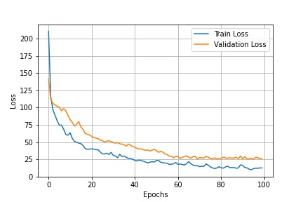
The YOLO v1 algorithm was modified to work correctly on the towing tank dataset. Thus, it needed to change the parameters for the input classes since the original model was trained on the Pascal VOC dataset containing 20 classes [3] while the towing tank dataset has only 5, and the dataset used for the object detection model was the initial towing tank dataset of 550 images. The results of the YOLO v1 model after 100 training epochs are shown in Figure bellow, where shows the training and validation loss of the model. The training and validation loss decreasing steadily through the training period as expected; although the validation loss has a minor gap from the training loss, it decreases almost at the same rate.
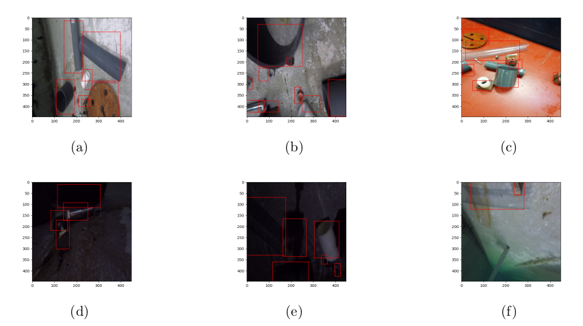
Additionally, the gigure bellow shows the resulted images when the model tested on some test images. The model performs quite accurately even in the cases with low light conditions, as in Figures d and e. Similarly, it has satisfactory results for images with many different objects, such as Figures a, b, and c, and can identify objects with transparent texture as in the figure f. For this model, the objective was to train an object detection model and study its behaviour and its viability to using it further in the project; thus, only the basics were implemented, and details such as the name of each identified object in an image will be in the next iteration when using the YOLO v4 architecture.
References
[1] J. Redmon, S. Divvala, R. Girshick, and A. Farhadi, You Only Look Once: Unified, Real-Time Object Detection , arXiv:1506.02640 [cs], May 2016, Accessed: Apr. 02, 2021. [Online]. Available: http://arxiv.org/abs/1506.02640